Statistics · Chapter 10

The Logic of Hypothesis Testing

Every interesting result comes with a nagging question: could that have happened by chance? A hypothesis test is a formal, honest way to answer it. You write down the boring explanation, you ask how surprising your data would be if that boring explanation were true, and you let the answer guide — not dictate — your decision. The machinery is simple arithmetic, but the reasoning is where students get lost, and where careless researchers publish nonsense. This chapter is about the reasoning: what a null hypothesis really claims, what a p-value really measures, what it emphatically does not measure, the two ways a test can be wrong, and why a "significant" finding can still be worth nothing at all.

By the end of this chapter you can

State a null hypothesis and an alternative hypothesis correctly, in terms of population parameters.
Choose between a one-tailed and a two-tailed alternative, and explain why the choice comes before the data.
Define the p-value as a conditional probability, and compute one from a test statistic.
Name the three or four things a p-value is routinely and wrongly claimed to mean.
Apply a significance level (α) to reach a decision, and use the language reject / fail to reject precisely.
Distinguish a Type I from a Type II error, and compute the power of a simple test.
Explain how sample size drives p-values, and why huge studies find trivial effects "significant."
State and check the assumptions a test rests on, and explain why a p-value is conditional on those too.
Report a result using an effect size and a confidence interval, and interpret that interval correctly.
Explain why a significant result does not by itself establish causation.

Section 1Null and alternative hypotheses

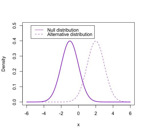
Two overlapping distributions showing the null hypothesis distribution and the alternative hypothesis distribution — **Reference.** The null distribution and the alternative distribution side by side — a hypothesis test asks which world your data look like they came from. Source and licence: see the figure credits

The courtroom, and why we start with the boring explanation

A hypothesis test is built like a criminal trial. The defendant is presumed innocent; the prosecution must produce evidence strong enough to overturn that presumption. In statistics, the presumption of innocence is called the null hypothesis, written H₀. It is always the dull, no-news, nothing-special explanation: the drug does nothing, the two groups are the same, the coin is fair, the population mean is exactly what everyone has always said it is.

Against it stands the alternative hypothesis, written H_a (some books write H₁). This is the claim you actually care about — the drug helps, the groups differ, the coin is loaded, the mean has shifted. Notice the asymmetry: the burden of proof sits entirely on H_a. If the evidence is weak, we do not conclude that H₀ is true; we simply say the prosecution failed. That asymmetry is the single most important idea in this chapter, and Section 3 returns to it.

Writing them correctly: four rules

Most errors in stating hypotheses are mechanical, and four rules fix nearly all of them.

Rule 1 — hypotheses are about parameters, never statistics. A hypothesis is a claim about the unknown population: μ (a population mean), p (a population proportion), σ (a population standard deviation), or the difference between two of those. It is never a claim about x̄ or the sample proportion p̂, because you can see those — there is nothing to hypothesize. Writing "H₀: x̄ = 20" is like hypothesizing about a number already printed in front of you.

Rule 2 — the equals sign lives in H₀. The null must pin the parameter to one specific value, because that value is what lets us build a probability model and compute anything at all. So H₀: μ = 20, never H₀: μ ≠ 20.

Rule 3 — H₀ and H_a must not overlap. Together they should cover the possibilities without both being true at once: μ = 20 versus μ ≠ 20, or μ ≤ 20 versus μ > 20.

Rule 4 — the direction is chosen before you look at the data. A two-tailed (two-sided) alternative, μ ≠ 20, says "different in either direction." A one-tailed (one-sided) alternative, μ > 20 or μ < 20, says "different in this specific direction," and it is only legitimate when the direction was decided in advance for a substantive reason — and when a difference in the other direction would be of no interest whatsoever. Peeking at the data, noticing the sample mean came out high, and then declaring a one-tailed test is a way of quietly doubling your chance of a false positive. When in doubt, go two-tailed.

Research question	H₀	H_a	Tails
Is the mean commute still 20 minutes?	μ = 20	μ ≠ 20	Two
Does the new curriculum raise scores above the old mean of 72?	μ ≤ 72	μ > 72	One (upper)
Is the defect rate below the promised 3%?	p ≥ 0.03	p < 0.03	One (lower)
Do two teaching methods differ in mean score?	μ₁ − μ₂ = 0	μ₁ − μ₂ ≠ 0	Two
Is the coin fair?	p = 0.5	p ≠ 0.5	Two

Setting up a real one

A transit office states that the mean one-way commute for students at a large institution is 20 minutes. You suspect it has crept upward, but you would also want to know if it had dropped, so you go two-tailed. You survey a random sample of n = 36 students and find x̄ = 22.4 minutes with s = 6.0 minutes.

The hypotheses, in the population's language, are

H₀: μ = 20 minutes versus H_a: μ ≠ 20 minutes.

Your sample came out 2.4 minutes high. That by itself proves nothing — samples wobble. The question the rest of this chapter answers is: if the mean really were 20, how often would a sample of 36 wobble this far? We carry this example through Sections 2, 3, and 4.

You can never "prove the null." A test can produce evidence against H₀, but no amount of unremarkable data proves that a parameter equals exactly 20.000… . Absence of evidence is not evidence of absence — especially with a small sample, where you might have missed a real difference entirely. That is why the verdict is "not guilty," not "innocent."

Interactive Write H₀ and Hₐ for six real claims — choosing the parameter, the null value, and the direction — and watch the null curve slide, the shaded tail flip, and the p-value recompute live, then see what it costs to pick the direction after looking at the data. Open full ↑

Key points

H₀ is the no-effect, no-difference explanation; H_a carries the claim and the burden of proof.
Hypotheses are statements about parameters (μ, p, σ), never about sample statistics.
The equality goes in H₀, because a specific value is what makes the probability calculation possible.
Choose one-tailed vs two-tailed before seeing the data; when unsure, use two-tailed.

Section 2The p-value

A distribution curve with the tail area beyond the observed test statistic shaded to represent the p-value — **Reference.** The p-value as a shaded tail area — the probability, under H₀, of a result at least as extreme as the one observed. Source and licence: see the figure credits

What it actually measures

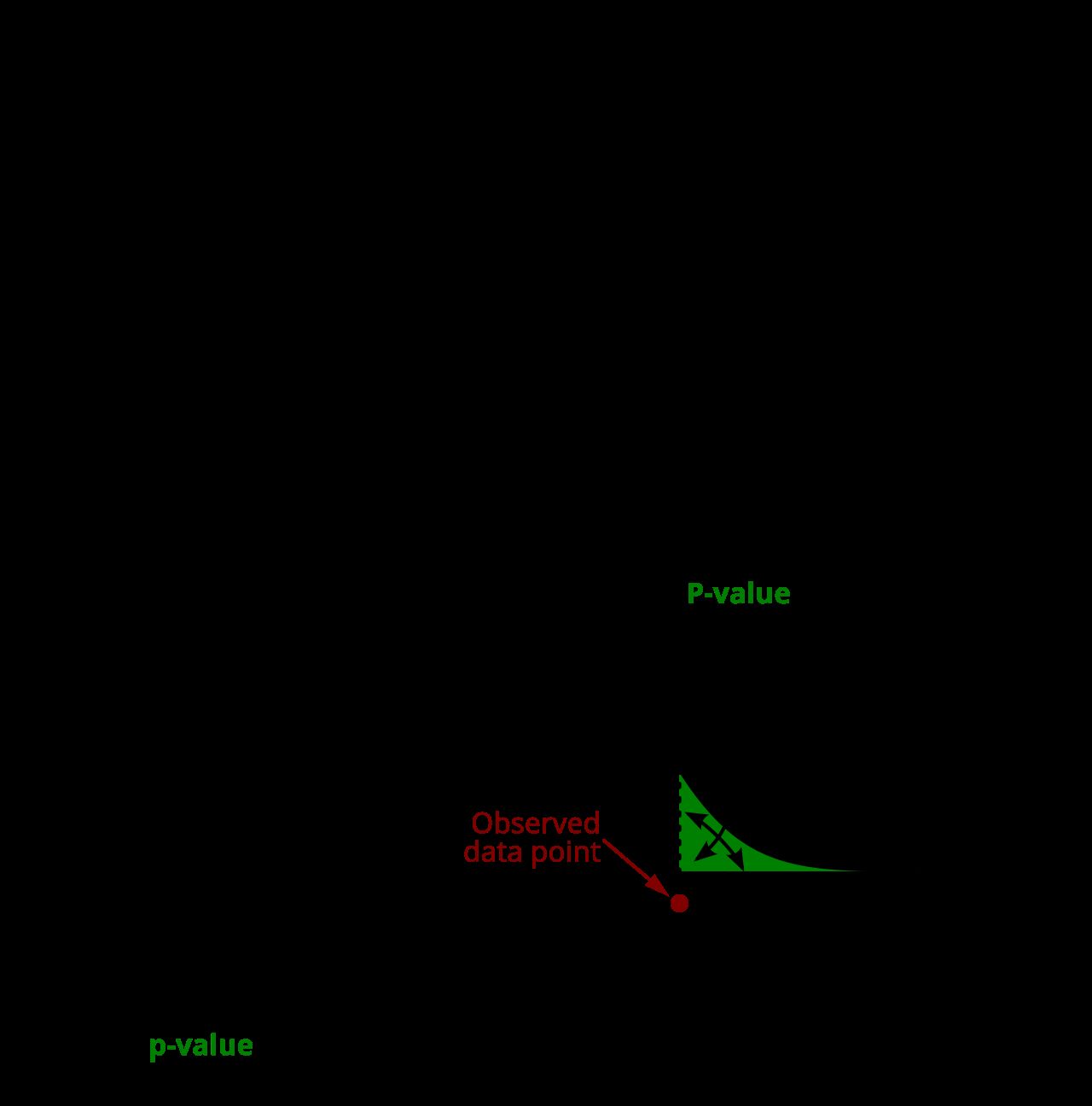
Assume, for the sake of argument, that H₀ is true. Under that assumption the sample statistic has a known sampling distribution — a predictable pattern of wobble. The p-value is the probability, computed inside that assumed world, of getting a result at least as extreme as the one you actually got.

Written as a conditional probability:

p = P( a test statistic at least this extreme | H₀ is true and the model's assumptions hold )

Read the vertical bar as "given." Everything to the right of it is assumed, not concluded. A small p-value means your data would be a rare event in the null world, which is grounds for doubting the null world. A large p-value means your data are perfectly ordinary there — unsurprising, and therefore uninformative.

Computing one, step by step

Back to the commutes: H₀: μ = 20, H_a: μ ≠ 20, with n = 36, x̄ = 22.4, s = 6.0.

Step 1 — standard error. The typical wobble of a sample mean is

SE = s / √n = 6.0 / √36 = 6.0 / 6 = 1.00 minute.

Step 2 — test statistic. Measure the gap between what you saw and what H₀ predicted, in units of that wobble:

t = (x̄ − μ₀) / SE = (22.4 − 20) / 1.00 = 2.40, with df = n − 1 = 35.

Your sample mean sits 2.40 standard errors above the null value.

Step 3 — tail area. On a t distribution with 35 degrees of freedom, the area beyond t = 2.40 in one tail is about 0.011. Because H_a is two-sided, "at least as extreme" includes results 2.40 SEs below 20 as well, so we double it:

p ≈ 2 × 0.011 = 0.022.

Step 4 — say it in English. If the true mean commute really were 20 minutes, then about 2.2% of random samples of 36 students would land at least 2.4 minutes away from 20 in one direction or the other. Our sample is in that unusual 2.2%. That is real, but not overwhelming, evidence against μ = 20.

What that calculation assumed

Every number above is conditional on a set of assumptions, and a one-sample t test has three that you are obliged to state and check before reporting anything:

Random sampling. The 36 commuters were drawn at random from the population the conclusion is about. A convenience sample breaks the link between the sampling distribution and reality, and no amount of arithmetic repairs it.
Independence. One person's commute tells you nothing about another's. Sampling 36 people who carpool together, or surveying the same person repeatedly, violates this and makes the standard error too small.
Approximate normality of the sampling distribution. Either the population of commute times is roughly normal, or n is large enough for the Central Limit Theorem to do the work. At n = 36 the t procedure is reasonably robust, but a strongly skewed population or a visible outlier — a single three-hour commute — can distort both x̄ and s. Plot the data before you trust the p-value.

The same three conditions carry through Sections 3, 4, and 5. When σ is known and used in place of s, as in the power calculation of Section 4, the test statistic becomes a z rather than a t, but the sampling, independence, and shape requirements are unchanged.

Four things a p-value is not

These misreadings are so common that they appear in press releases, textbooks, and published papers. Learn them as a list of things you will never say.

People say	Why it is wrong	What is actually true
"p = 0.022, so there is a 2.2% chance the null is true."	Reverses the conditioning. The p-value is P(data \| H₀), not P(H₀ \| data).	P(H₀ \| data) cannot be computed without prior probabilities; classical testing never supplies them.
"There is a 97.8% chance the alternative is true."	Same reversal, mirrored. 1 − p is not the probability of H_a.	1 − p is just the non-tail area of the null distribution. It says nothing about H_a.
"p = 0.022 means the effect is big."	Confuses evidence with magnitude. A tiny effect gets a small p-value if n is huge.	Magnitude is reported by an effect size and a confidence interval (Section 5).
"p = 0.022 means it will replicate 97.8% of the time."	Replication probability depends on the true effect and the new study's power, not on p.	A study with p just under 0.05 often replicates barely half the time.
"p = 0.30 proves there is no effect."	A large p-value is a failure to detect, not a demonstration of absence.	An underpowered study returns large p-values even when the effect is real (Section 4).

One more caution hides in the fine print of the definition. The p-value assumes H₀ and every modeling assumption: random sampling, independence, the right distributional shape, no selective reporting. A small p-value is evidence that something in that whole package is wrong. If your sample was a convenience sample of your friends, the thing that is wrong may not be H₀.

The bar in P(A | B) points one way. The probability that someone is a professional basketball player given that they are over 7 feet tall is high. The probability that someone is over 7 feet tall given that they are a professional basketball player is a very different number. A p-value is the second kind of statement about your data — and people habitually read it as the first kind of statement about your hypothesis.

Interactive Drag your result along the null distribution to shade the tail and watch the p-value recompute, then run thousands of simulated studies in a world where the null is true and count the extreme ones yourself. Open full ↑

Key points

The p-value is P(result this extreme or more | H₀ true and assumptions hold).
Compute it in three moves: standard error → test statistic → tail area, doubling the tail for a two-sided H_a.
It is not the probability the null is true, not the probability of replication, and not a measure of effect size.
A small p-value indicts the whole model, not just H₀ — check your sampling and assumptions first.

Section 3Significance and decisions

A normal curve divided into a central non-rejection region and shaded rejection regions in the tails — **Reference.** Rejection regions in the tails versus the non-rejection region in the middle — the geometry of a significance level. Source and licence: see the figure credits

Alpha: an error budget you set in advance

A p-value is a continuous measure of surprise. Sooner or later, though, somebody has to do something — approve the drug, change the curriculum, keep the old machine. Turning a continuous measure into a yes/no decision requires a threshold, and that threshold is the significance level, written α.

α is not a law of nature; it is a choice about how much false-alarm risk you are willing to tolerate. Setting α = 0.05 means: if H₀ is true, I accept a 5% chance of wrongly rejecting it. Fields that can afford a few false alarms use 0.05. Fields where a false alarm is catastrophic or where thousands of tests are run at once — genetics, particle physics — use 0.01, 10⁻⁶, or smaller. The one non-negotiable rule is that α is fixed before you see the data. Choosing α after the p-value arrives is not statistics; it is bookkeeping in reverse.

The decision rule, both ways

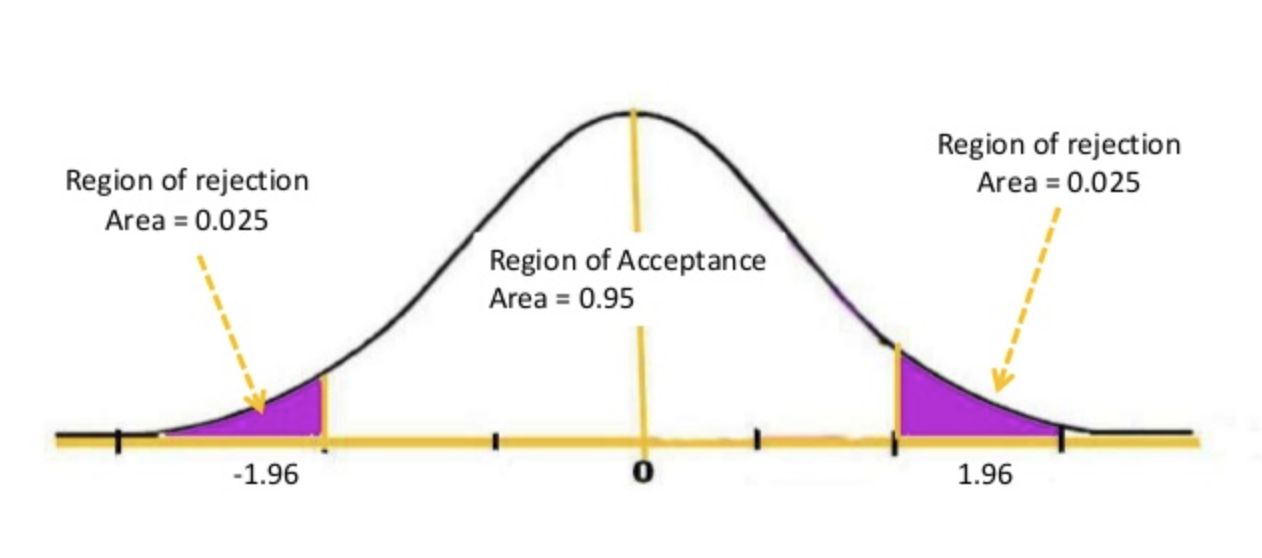
The rule itself is one line: if p ≤ α, reject H₀; if p > α, fail to reject H₀. An equivalent route compares the test statistic to a critical value instead, which is the picture the figure above shows: the tails cut off by α form the rejection region, and a statistic landing there triggers rejection.

Our commute study, with α = 0.05 set in advance:

p-value route. p ≈ 0.022. Since 0.022 ≤ 0.05, reject H₀.

Critical-value route. With df = 35 and a two-tailed α = 0.05, the critical value is t* = 2.030, so the rejection region is t < −2.030 or t > 2.030. Our t = 2.40 lands beyond 2.030, so we reject H₀. Same verdict, necessarily — the two routes are the same statement seen from two sides.

Now suppose the sample mean had been 21.6 instead of 22.4. Then

t = (21.6 − 20) / 1.00 = 1.60, and with df = 35 the two-tailed p ≈ 0.119.

Here 0.119 > 0.05, and 1.60 does not reach 2.030, so we fail to reject H₀. Note carefully what we have and have not learned. The sample mean was still 1.6 minutes above 20. We have not shown the commute is 20 minutes. We have shown that a wobble this size is unremarkable in a sample of 36 — so this study cannot tell the difference between "no change" and "a change we were too small to detect."

Say it right

Outcome	Say this	Never say this
p ≤ α	"Reject H₀." / "The result is statistically significant at α = 0.05."	"H_a is proven." / "The null is false."
p > α	"Fail to reject H₀." / "There is insufficient evidence of a difference."	"Accept H₀." / "We proved there is no difference."
Any outcome	Report the estimate, the interval, and the exact p-value.	"p < 0.05" with no effect size.
p = 0.051	"Weak evidence; the interval runs from … to …"	"No effect." / "Trending toward significance."

Why the fuss about "fail to reject" instead of "accept"? Because the test was never designed to gather evidence for H₀. The whole apparatus — sampling distribution, tail area, rejection region — was built inside the assumption that H₀ is true, so it can only ever tell you whether that assumption strains. It has no mechanism for confirming it. A jury that acquits has not proven innocence; it has found the evidence insufficient.

0.049 and 0.051 are the same result. α = 0.05 is a convention, not a cliff. Two studies on opposite sides of it differ by an amount no scientist could care about, yet one gets called "significant" and the other "null." Treat α as a decision rule for when you must act, and treat the p-value itself as what it is — a continuous, and rather noisy, measure of surprise.

Interactive Drag the significance level across a live two-tailed z-test and watch one unchanged p-value flip from "fail to reject" to "reject" — then see the long-run error rate that your choice of alpha actually buys. Open full ↑

Key points

α is the false-alarm rate you agree to tolerate, chosen before the data arrive.
Decision rule: p ≤ α → reject H₀; p > α → fail to reject. The critical-value route always agrees.
"Fail to reject" ≠ "accept" — the test cannot supply evidence in favor of the null.
Significance is a threshold crossing, not a measurement; report the estimate and interval alongside it.

Section 4Type I and Type II errors

Two overlapping distributions with shaded areas labelled for significance level and statistical power — **Reference.** Significance level and power drawn together — the null distribution's tail is α, the alternative distribution's overlap is β, and what remains is power. Source and licence: see the figure credits

Two ways to be wrong

Reality has two states and your test has two verdicts, so there are four combinations — two right, two wrong.

	H₀ is actually true	H₀ is actually false
Reject H₀	Type I error — false alarm. Probability = α.	Correct decision. Probability = 1 − β = power.
Fail to reject H₀	Correct decision. Probability = 1 − α.	Type II error — missed detection. Probability = β.

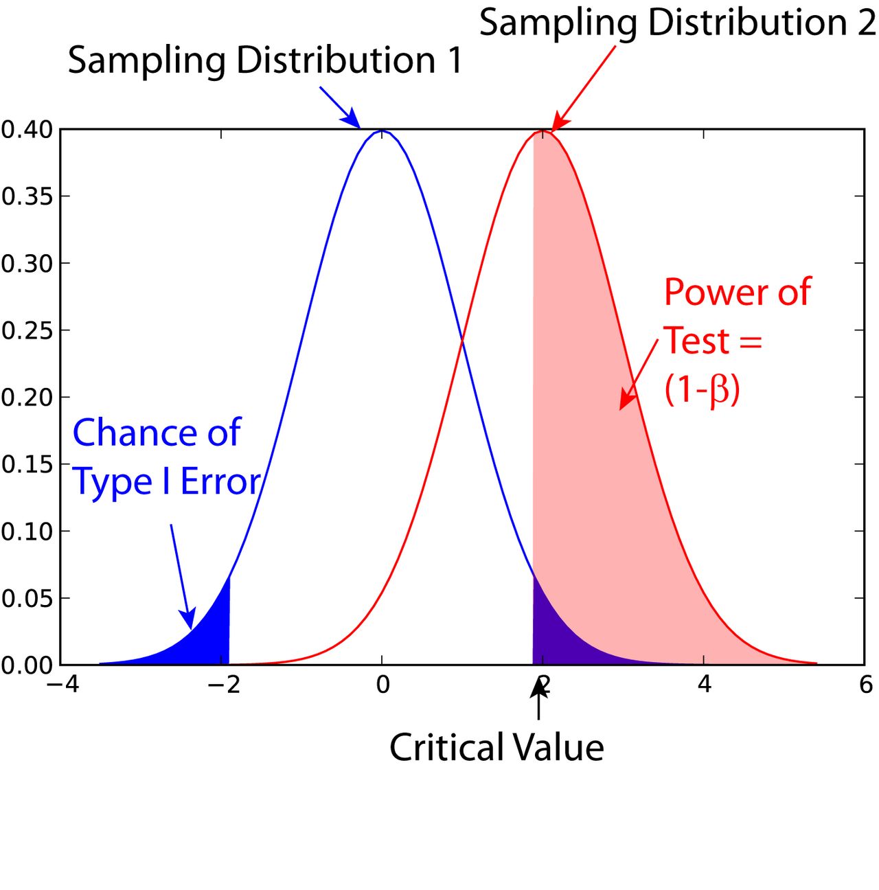
A Type I error is convicting the innocent: declaring an effect that is not there. You control it directly, because α is its probability — that is what setting α = 0.05 buys you. A Type II error is acquitting the guilty: missing an effect that is genuinely there. Its probability, β, you do not set directly; it falls out of how big the real effect is, how noisy your measurements are, how large your sample is, and what α you chose.

Power is the good half of that second column: power = 1 − β, the probability that your study detects an effect of a given size when that effect is real. Power is a property of a study design plus a specific alternative — there is no such thing as "the power of a test" without naming the effect size you want to catch.

Computing power, with numbers

Return to the commute study. To keep the arithmetic clean, suppose the population standard deviation is known to be σ = 6.0 minutes, so we can work with the standard normal. Test H₀: μ = 20 against H_a: μ ≠ 20 at α = 0.05 with n = 36. Ask: if the true mean is really 21.5 minutes, what is the chance we detect it?

Step 1 — find the rejection region in real units. SE = σ/√n = 6.0/6 = 1.00. A two-tailed α = 0.05 uses z* = 1.96, so we reject whenever

x̄ > 20 + 1.96(1.00) = 21.96 or x̄ < 20 − 1.96(1.00) = 18.04.

Step 2 — move into the true world. If μ = 21.5, then x̄ is centered at 21.5 with the same SE = 1.00. Standardize both boundaries against 21.5:

upper: z = (21.96 − 21.5)/1.00 = 0.46 → P(Z > 0.46) = 1 − 0.6772 = 0.3228

lower: z = (18.04 − 21.5)/1.00 = −3.46 → P(Z < −3.46) = 0.0003

Step 3 — add. Power = 0.3228 + 0.0003 ≈ 0.32, so β ≈ 1 − 0.32 = 0.68.

Read that again, because it is sobering. If the commute truly has risen by a minute and a half, this 36-person study misses it roughly 68% of the time. Most of its "no significant difference" conclusions would be wrong.

Step 4 — fix it with sample size. Quadruple n to 144. Then SE = 6.0/√144 = 6.0/12 = 0.50, and we reject when x̄ > 20 + 1.96(0.50) = 20.98 (or below 19.02). Standardizing against the true 21.5:

z = (20.98 − 21.5)/0.50 = −1.04 → P(Z > −1.04) = 0.8508

The lower boundary contributes essentially nothing, so power ≈ 0.85. Quadrupling n halved the standard error and took power from 32% to 85%. This is exactly what a power analysis does before a study is run: pick the smallest effect worth detecting, pick a target power (0.80 is the usual floor), and solve for the n you need.

The four levers, and the trade-off

Lever	Move it this way	Effect on power	Cost
Sample size n	Increase	Rises — SE shrinks like 1/√n	Time, money, participants
True effect size	Larger real difference	Rises	Not yours to choose
Variability σ	Decrease (better measurement, tighter design)	Rises	Effort, instrumentation
Significance level α	Increase (0.01 → 0.05)	Rises	More Type I errors

The last row is the central tension of the whole framework. Holding everything else fixed, the only way to make Type I errors rarer is to shrink the rejection region, which makes Type II errors more common — and vice versa. You cannot reduce both by adjusting α. The one lever that improves both at once is a bigger, cleaner sample, which is why sample size is the design question that matters most.

Which error is worse depends entirely on context, and that is a judgment about consequences, not statistics. In screening for a treatable cancer, a Type II error (missing a real case) is far worse than a Type I error (a false alarm resolved by a follow-up test), so screening tests are deliberately tuned toward high power. In a criminal trial, the system deliberately accepts many Type II errors to avoid Type I errors.

A nonsignificant result from an underpowered study means almost nothing. Before you take "no difference was found" seriously, ask what effect the study could have detected. If its power against a meaningful effect was 30%, its failure to find one is roughly as informative as a coin flip — and reporting it as evidence of no effect is a genuine error.

Interactive Tap through the four-cell error matrix while three live sliders — sample size, true effect, and alpha — recompute the overlapping null and alternative distributions, a power curve, and 200 simulated studies, showing why a bigger sample cures misses but never false alarms. Open full ↑

Key points

Type I error = rejecting a true H₀ (false alarm); its probability is exactly α.
Type II error = failing to reject a false H₀ (missed detection); its probability is β.
Power = 1 − β, always stated against a specific effect size; 0.80 is the conventional minimum.
Lowering α raises β; only larger n or less variability improves both kinds of error at once.

Section 5Statistical versus practical significance

A point estimate shown with a confidence interval around it on a number line — **Reference.** A point estimate with its confidence interval — the report that answers "how big?", which a p-value alone never does. Source and licence: see the figure credits

Sample size manufactures significance

Look once more at the test statistic and notice what is in the denominator:

t = (x̄ − μ₀) / (s/√n)

Hold the numerator fixed — the same real difference — and let n grow. The denominator shrinks toward zero, so t grows without bound and the p-value slides toward zero. Any difference from H₀, no matter how minuscule, becomes statistically significant at a large enough sample size. Statistical significance answers "can we tell this is not exactly zero?" It never answers "is it big enough to care about?"

A worked pair: the significant triviality and the invisible whale

Study A. A supplement company follows n = 40,000 participants and records each one's weight change over six months, testing H₀: μ = 0 against a two-sided alternative. The mean change is 0.20 pounds, with s = 10 pounds. (Because this is a single sample of 40,000 changes, the one-sample formula SE = s/√n applies; comparing two separate groups would require the two-sample standard error instead.)

SE = s/√n = 10/√40000 = 10/200 = 0.05

t = 0.20 / 0.05 = 4.00, giving p < 0.0001 — wildly "significant."

95% confidence interval: 0.20 ± 1.96(0.05) = 0.20 ± 0.098 → (0.10, 0.30) pounds.

Effect size (Cohen's d) = difference / s = 0.20/10 = 0.02, which is negligible by any standard.

The interval is the punchline. We are confident the true effect is somewhere between a tenth and three tenths of a pound. It is real, it is not zero, and it is completely worthless to a person trying to lose weight. Significant, and trivial.

Study B. A small trial follows n = 25 participants over the same six months and tests the same H₀: μ = 0. The mean weight change is 4.0 pounds, again with s = 10 pounds.

SE = 10/√25 = 10/5 = 2.00

t = 4.0/2.00 = 2.00, df = 24, two-tailed p ≈ 0.057 — "not significant."

95% CI: 4.0 ± 2.064(2.00) = 4.0 ± 4.13 → (−0.13, 8.13) pounds.

Effect size d = 4.0/10 = 0.40, a small-to-moderate effect worth chasing.

Study B failed the α = 0.05 threshold, but its interval is compatible with an eight-pound benefit. The honest conclusion is not "the supplement does not work" — it is "this study was too small to say." Study A is the more significant result and the less important one; Study B is the less significant result and the more promising one.

	Practically important	Practically trivial
Statistically significant	The goal — a real, meaningful effect, well measured.	Huge n detecting a difference nobody would act on (Study A).
Not statistically significant	Promising but underpowered — wide interval, needs a bigger study (Study B).	Genuinely uninteresting, or genuinely no effect. The interval tells you which.

What to report instead

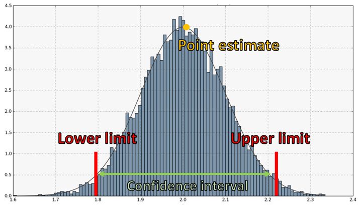
A complete result has three parts, and only the third is the p-value: the estimate (how big), the interval (how precisely we know it), and the test (how surprising it would be under the null). Study A reported properly reads: "0.20 lb, 95% CI (0.10, 0.30), d = 0.02, p < 0.0001" — and no reader is fooled for a second.

A fourth caution belongs with the other three, because it is the one most likely to survive into a headline. A significant test result does not establish that anything caused anything. Causal standing comes from the design — randomized assignment, a control condition, and control of confounding variables — not from the size of a test statistic. Study A's participants chose to take a supplement; whatever separates them from people who did not may also separate them in diet, income, or exercise, and the p-value cannot tell those explanations apart. The same rule holds for an observed association between two measured variables: a small p-value on a correlation says the association is unlikely to be zero, and nothing more. Significance answers "is this pattern distinguishable from noise?" Only the design answers "why is the pattern there?"

One last precision point, because it is misstated constantly. A 95% confidence interval is a statement about the procedure, not about this one interval. It means: if you repeated the whole study endlessly and built an interval each time by this method, about 95% of those intervals would contain the true parameter. It does not mean there is a 95% probability that the true parameter lies inside the particular interval you just computed. That interval either contains μ or it does not; the parameter is a fixed number, not a random one. The 95% describes the long-run reliability of the machine that produced it.

Ask "how big?" before you ask "is it significant?" Decide in advance what difference would be large enough to change what you do — the minimum important difference — and then check whether your confidence interval excludes it. A test tells you whether zero is plausible. Only the interval tells you whether the effect clears the bar you actually care about.

Interactive Hold a trivially small true drug effect fixed and slide the sample size from 10 to 500,000 — a live two-tailed z-test drives p below 0.05 and on to 10⁻¹²³, while the overlapping population curves, Cohen's d, and the confidence interval show the effect never became worth treating. Open full ↑

Key points

Because SE = s/√n, large samples make any nonzero difference statistically significant.
Statistical significance answers "not zero?"; practical significance answers "big enough to matter?"
Report an effect size and a confidence interval alongside the p-value, never the p-value alone.
A 95% CI describes the long-run success rate of the procedure, not a 95% probability for this specific interval.
Significance never establishes causation — that comes from randomization and control in the design, not from the p-value.

The chapter in one breath

H₀ is the no-effect explanation and carries the equality; H_a is your claim and carries the burden of proof. Both are statements about parameters, and the number of tails is chosen before you look.
The p-value is P(a result this extreme or more | H₀ true and assumptions hold) — computed as standard error, then test statistic, then tail area.
A p-value is not the probability the null is true, not the probability of replication, and not a measure of how big the effect is.
α is a false-alarm budget fixed in advance; p ≤ α means reject H₀, p > α means fail to reject — never "accept."
A Type I error (probability α) is a false alarm; a Type II error (probability β) is a miss; power = 1 − β is stated against a specific effect size.
Shrinking α inflates β and vice versa; only larger n or less variability improves both, which is why power analysis precedes data collection.
Because SE shrinks with √n, a large enough study makes any trivial difference "significant" — and a small study can miss a large one.
Every p-value is conditional on the test's assumptions — random sampling, independence, and adequate normality — as well as on H₀; state and check them before reporting.
Report the estimate, the confidence interval, and the effect size; a 95% CI describes the long-run behavior of the procedure, not this interval's chance of being right.
Statistical significance is never evidence of causation; only the design — randomization, control, and handling of confounders — can support a causal claim.

ReferenceWords worth knowing

A quick reference for the vocabulary in this chapter. The definitions are worded to be precise rather than casual — in hypothesis testing, the casual wording is usually the wrong one.

Alpha (α, significance level): The maximum probability of a Type I error you agree to tolerate, fixed before the data are seen. Commonly 0.05, but the value should suit the consequences of a false alarm.
Alternative hypothesis (H_a): The statement about a population parameter that contradicts H₀ and expresses the claim under investigation; it may be two-sided (≠) or one-sided (> or <).
Assumptions (of a test): The conditions a test's mathematics depends on — for a one-sample t test: random sampling, independent observations, and a sampling distribution close enough to normal. A p-value is conditional on these as well as on H₀, so they must be stated and checked before the result is reported.
Beta (β): The probability of a Type II error — failing to reject a false H₀. Not set directly; it depends on effect size, variability, sample size, and α.
Confidence interval: A range of parameter values produced by a procedure that, in repeated use, captures the true parameter a stated proportion of the time (e.g., 95%). It quantifies precision, not the probability of one particular interval.
Critical value: The cutoff on the test statistic's null distribution that bounds the rejection region for a given α (for example, z* = 1.96 for a two-tailed test at α = 0.05).
Effect size: A measure of the magnitude of a difference or relationship, independent of sample size — for instance Cohen's d, the mean difference divided by the standard deviation.
Fail to reject: The verdict when p > α: the evidence is insufficient to overturn H₀. It is not a conclusion that H₀ is true.
Null hypothesis (H₀): The default statement of no effect, no difference, or no change, pinned to a specific parameter value so that a sampling distribution can be constructed.
One-tailed (one-sided) test: A test whose alternative specifies a direction; the entire rejection region sits in one tail. Legitimate only when the direction is chosen in advance on substantive grounds.
Parameter: A fixed numerical characteristic of a population, such as μ, σ, or p. Hypotheses are always about parameters.
Power: 1 − β: the probability of correctly rejecting H₀ when a specified alternative is true. Rises with larger n, larger true effects, smaller variability, and larger α.
Practical significance: Whether an effect is large enough to matter in the real world, judged against a minimum important difference — a separate question from statistical significance.
p-value: The probability, assuming H₀ and all model assumptions are true, of obtaining a test statistic at least as extreme as the one observed.
Rejection region: The set of test-statistic values, determined by α, that lead to rejecting H₀; the shaded tail area(s) of the null distribution.
Sampling distribution: The distribution a statistic would follow across all possible samples of a given size; the mathematical object that makes a p-value computable.
Standard error (SE): The standard deviation of a sampling distribution. For a mean, SE = s/√n (or σ/√n when σ is known).
Statistic: A number computed from a sample, such as x̄ or s; used to estimate a parameter and to test hypotheses about it.
Statistically significant: Describes a result whose p-value falls at or below the pre-set α, meaning the data would be unusual if H₀ were true. It implies nothing about magnitude.
Test statistic: A standardized measure of the distance between the observed data and what H₀ predicts, expressed in standard errors — for example t = (x̄ − μ₀)/(s/√n).
Two-tailed (two-sided) test: A test whose alternative is simply "different," splitting the rejection region between both tails; the safe default when no direction was specified beforehand.
Type I error: Rejecting H₀ when it is actually true — a false positive. Its probability is exactly α.
Type II error: Failing to reject H₀ when it is actually false — a false negative, or missed detection. Its probability is β.

Check yourself

1. A manufacturer claims its bags average 500 grams. You suspect underfilling. Write H₀ and H_a, and say how many tails you would use and why.

H₀: μ ≥ 500 grams; H_a: μ < 500 grams — one-tailed (lower). The suspicion of underfilling is directional and stated before the data are collected, and overfilling would not be a complaint, so a lower one-tailed test is legitimate. Note the hypotheses are about μ, the population mean, and the equality lives on the null side.

2. What is wrong with writing "H₀: x̄ = 500"?

Hypotheses must be about parameters, not statistics. You already know x̄ — you computed it from your sample — so there is nothing to hypothesize. The unknown quantity is the population mean μ, and that is what H₀ must be about.

3. A study reports p = 0.03. A colleague says, "So there is a 3% chance the null hypothesis is true." Correct them precisely.

The p-value is P(data this extreme or more | H₀ true), not P(H₀ true | data). It says that if the null were true, results this extreme would occur about 3% of the time. Computing the probability that H₀ is true would require prior probabilities, which classical hypothesis testing never supplies.

4. A sample of n = 64 gives x̄ = 103 with s = 16, testing H₀: μ = 100 two-sided. Compute SE and the test statistic.

SE = 16/√64 = 16/8 = 2.00; t = (103 − 100)/2.00 = 1.50 with df = 63. The sample mean sits 1.5 standard errors above the null value; the two-tailed p-value is roughly 0.14, so at α = 0.05 you would fail to reject H₀.

5. Why do we say "fail to reject H₀" rather than "accept H₀"?

The entire calculation is performed inside the assumption that H₀ is true, so the test can only detect strain on that assumption — it has no mechanism for confirming it. A large p-value may mean there is no effect, or it may mean the study was too small to detect a real one. Like a jury acquitting for lack of evidence, we decline to convict without declaring innocence.

6. Define Type I and Type II errors and give the probability of each.

Type I = rejecting a true H₀ (false positive), probability α. Type II = failing to reject a false H₀ (false negative), probability β. You set α directly; β is a consequence of effect size, variability, sample size, and α.

7. A researcher lowers α from 0.05 to 0.01 to be "more careful." What happens to the two error probabilities, and to power?

Type I error probability falls to 0.01, but β rises and power falls. Shrinking the rejection region makes false alarms rarer and missed detections more common. The only lever that improves both at once is a larger sample (or less measurement noise).

8. Testing H₀: μ = 20 against a two-sided alternative with σ = 6, n = 36, α = 0.05, the rejection region is x̄ > 21.96 or x̄ < 18.04. If the true mean is 21.5, what is the power?

About 0.32. SE = 6/√36 = 1.00. Standardizing the upper boundary against the true mean: z = (21.96 − 21.5)/1.00 = 0.46, and P(Z > 0.46) = 0.3228. The lower boundary gives z = −3.46, contributing about 0.0003. Power ≈ 0.32, so β ≈ 0.68 — the study misses this effect about two thirds of the time.

9. In Question 8, the sample size is raised to n = 144. Show why power rises to roughly 0.85.

SE = 6/√144 = 0.50, so the upper cutoff becomes 20 + 1.96(0.50) = 20.98; standardizing against 21.5 gives z = (20.98 − 21.5)/0.50 = −1.04, and P(Z > −1.04) = 0.8508. Quadrupling n halved the standard error, which pulled the cutoff much closer to the true mean and raised power from 32% to about 85%.

10. A single sample of n = 40,000 participants has a mean weight change of 0.20 lb with s = 10 lb, tested against H₀: μ = 0, and reports p < 0.0001. Compute the 95% CI and Cohen's d, then interpret.

SE = 10/√40000 = 0.05; CI = 0.20 ± 1.96(0.05) = (0.10, 0.30) lb; d = 0.20/10 = 0.02. The effect is real and precisely measured but negligible — a tenth to three tenths of a pound, and an effect size of 0.02. This is statistical significance without practical significance, produced by an enormous sample.

11. A study with n = 25 finds a mean weight change of 4.0 lb, s = 10 lb, p ≈ 0.057, 95% CI (−0.13, 8.13). Is "the treatment does not work" a fair conclusion?

No. The result is nonsignificant, but the interval is compatible with a benefit of up to about 8 pounds. SE = 10/√25 = 2.00 and t = 4.0/2.00 = 2.00 with df = 24, so this simply failed to clear α = 0.05. With d = 0.40, the honest conclusion is that the study was too small to decide — not that the effect is absent.

12. State exactly what "95% confidence" means, and say what it does not mean.

It means that if the study were repeated indefinitely and an interval built each time by this procedure, about 95% of those intervals would contain the true parameter. It does not mean there is a 95% probability that the parameter lies inside the one interval you computed. The parameter is a fixed number; that interval either contains it or it does not. The 95% is a property of the method, not of this result.

Previous← Confidence Intervals NextOne-Sample Tests →